Omega3P
Omega3P computes the resonant modes of an RF cavity: the eigenfrequencies, the quality factors, and the electromagnetic field distribution of each mode. It is the most widely used ACE3P module and the starting point for most other analyses, since Track3P, TEM3P, and the acdtool RF post-processor all consume its output.
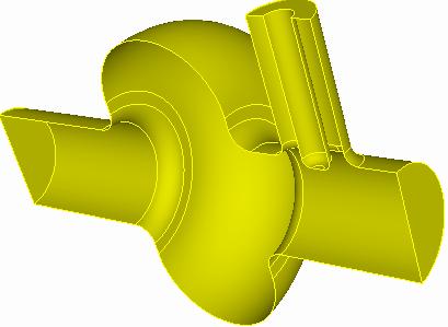
Cavities analyzed in the tutorials: rounded pillbox, coax coupler, waveguide coupler with lossy load, and a traveling-wave cell.
What it solves
In the frequency domain, Maxwell's equations in a source-free cavity reduce to the vector wave equation for the electric field:
Discretizing with high-order Nédélec vector finite elements gives a generalized eigenvalue problem \(K\mathbf{x} = \lambda M\mathbf{x}\) with \(\lambda = \omega^2\). Omega3P handles three cases:
| Case | Eigenvalue | When |
|---|---|---|
| Lossless, closed cavity | Real | Perfect electric or magnetic walls, periodic boundaries. Wall loss and Q0 are computed afterward by perturbation from the surface conductivity. |
| Open or lossy cavity | Complex | Waveguide ports, absorbing boundaries, lossy dielectrics, surface impedance. The imaginary part gives the external or dielectric Q. |
| Multiple ports with different cutoffs | Nonlinear | Each port adds a frequency-dependent term. Solved with the CORK rational Krylov method. |
The frequency is \(f = \omega / 2\pi\) and, for a complex eigenvalue, \(Q = \mathrm{Re}(f) / 2\,\mathrm{Im}(f)\).
Capabilities
- Perfect electric and magnetic boundary conditions for symmetry reduction
- Periodic boundaries with an arbitrary phase advance, for dispersion curves of traveling-wave structures
- Waveguide ports with modal expansion, for coupler external Q
- Absorbing boundaries for simple beam-pipe truncation
- Volume materials with complex permittivity, for loads and windows
- Surface conductivity for wall-loss Q0, and surface impedance for coatings
- Finite-element orders 1 through 6 on curved tetrahedra
- Adaptive mesh refinement driven by an error estimate
- Checkpoint and restart of long eigensolves
Input file
The input <project>.omega3p uses the common blocks plus EigenSolver and, for open cavities, one Port block per port. A complete lossless example:
ModelInfo : {
  File: ./pillbox4.ncdf
  BoundaryCondition : {
    Magnetic: 1, 2
    Exterior: 6
  }
  SurfaceMaterial : {
    ReferenceNumber: 6
    Sigma: 5.8e7
  }
}

FiniteElement: {
  Order:           2
  CurvedSurfaces: on
}

EigenSolver : {
  NumEigenvalues: 2
  FrequencyShift:  1.0e9
}

PostProcess : {
  Toggle: on
  ModeFile: mode
}
EigenSolver block
| Key | Default | Meaning |
|---|---|---|
NumEigenvalues |
1 | How many modes to find, counting upward in frequency from FrequencyShift |
FrequencyShift |
10 GHz | Target frequency. The solver finds the modes nearest to and above this value. Set it a little below the lowest mode you want. |
FrequencyShiftImag |
0 | Imaginary part of the shift, for complex problems |
Tolerance |
1e-8 | Relative residual for eigenpair convergence |
MaxIterations |
200 | Krylov iteration limit |
SolverMode |
automatic |
Choose the algorithm explicitly: Arnoldi, InexactLanczos, ESIL, SOAR, CORK. Automatic picks by problem type. |
CORK |
Sub-block with TargetFrequencyMin, TargetFrequencyMax, TargetFrequencyImag, ApproxTolerance, ApproxMaxDegree for the nonlinear solver. See Tutorial 2. |
The full list, including adaptive refinement and matrix dump options, is in the Omega3P keyword reference, and every block is described key by key in the Omega3P command syntax.
When is a multi-port problem quadratic, and when nonlinear?
With waveguide ports the eigenproblem is quadratic, and the default solver handles it, when every port loads one mode and all ports share the same cutoff frequency. The CW23 slides give the example of a pillbox whose waveguide coupler and both beam-pipe ends are all declared Waveguide with one mode each. When ports have different cutoffs, or several modes per port, the problem is nonlinear and there are three options in increasing accuracy and cost: the 1D Absorbing boundary (an approximation), a PML (a good approximation, see the command syntax), or the CORK nonlinear solver (accurate but harder to converge).
Port block
Port : {
  ReferenceNumber : 7     // sideset of the port surface
  NumberOfModes : 1       // waveguide modes to load at this port
}
A surface listed under Waveguide in BoundaryCondition must have a matching Port block, or Omega3P loads one mode by default. The port is treated as matched for every loaded mode. Choosing how many modes to load is discussed in Tutorial 2.
Output
Results go into omega3p_results/ next to the input file.
| File | Content |
|---|---|
omega3p.out |
Full log: parsed input, mesh statistics, DOF count, iteration history, and a Mode block per eigenpair with Frequency, QualityFactor, ExternalQ, TotalEnergy, PowerLoss, and the field file name |
omega3p.log |
Shorter progress log |
omega3p.warn |
Warnings. Read this if a result is unexpected. |
omega3p.l0.m0000.<freq>.mod |
Field file for mode 0 at refinement level 0. One per mode. For complex problems the name carries R<real>.I<imag>. |
2dports.log |
Cutoff frequencies and types of the waveguide modes computed on each port surface |
VECTOR/ |
Raw eigenvectors |
A typical mode summary:
Mode : {
    TotalEnergy : 4.2137588190101e-12 , 0
    ExternalQ : 267.27097453785
    QualityFactor : 26238.857067312
    File : omega3p_results/omega3p.l0.m0000.R1.1762928e+09.I2.2005621e+06.mod
    PowerLoss : 1.1869161916105e-06
    Frequency : 1176292763.7678 , 2200562.1182804
}
QualityFactor is the wall-loss Q0 from SurfaceMaterial. ExternalQ is from the ports and is only present for complex problems. The two Frequency numbers are the real and imaginary parts in hertz.
Tutorials
- Pillbox cavity: the complete workflow from Cubit journal to R/Q, plus a mesh convergence study.
- Coax and waveguide couplers: waveguide ports, external Q, and the nonlinear eigenproblem with two ports.
- Lossy load and periodic boundaries: multiple materials with complex permittivity, and a dispersion point of a disk-loaded structure.
Post-processing with acdtool postprocess rf has its own page: Post-processing.