User Guide
The Trace Window
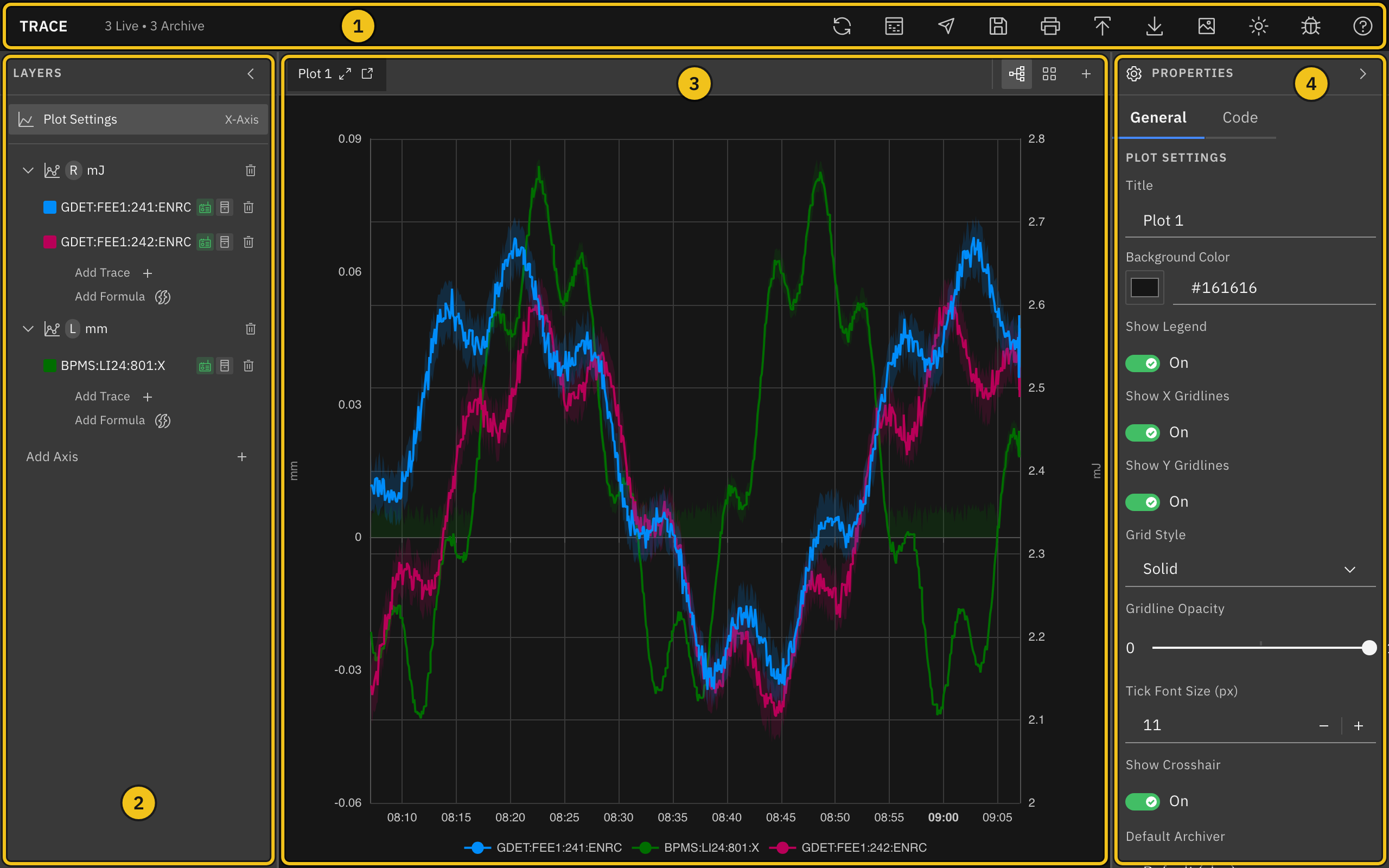
The Trace window has four areas:
- ① Header — the toolbar for saving, exporting, printing, and other actions. The counter next to SLAC Trace shows how many traces on the current plot use live and archive data.
- ② Layers — the plot's axes and the traces on each axis. Click an item to edit it.
- ③ Plot area — the plot itself, with plot tabs and view controls above it.
- ④ Properties — settings for whatever is selected in Layers: the plot, an axis, or a trace.
Resize and Collapse Panels
Drag the border between two panels to resize them. Click the chevron in the Layers or Properties header to collapse that panel to a thin strip, and click the strip to open it again. Useful when you want more room for the plot.
Plot a PV
Every plot starts with one empty Y-axis. To plot a process variable (PV), add a trace to an axis and choose the PV it should follow. New traces show both archived and live data, so the plot fills the whole time range and keeps updating.
Workflow:
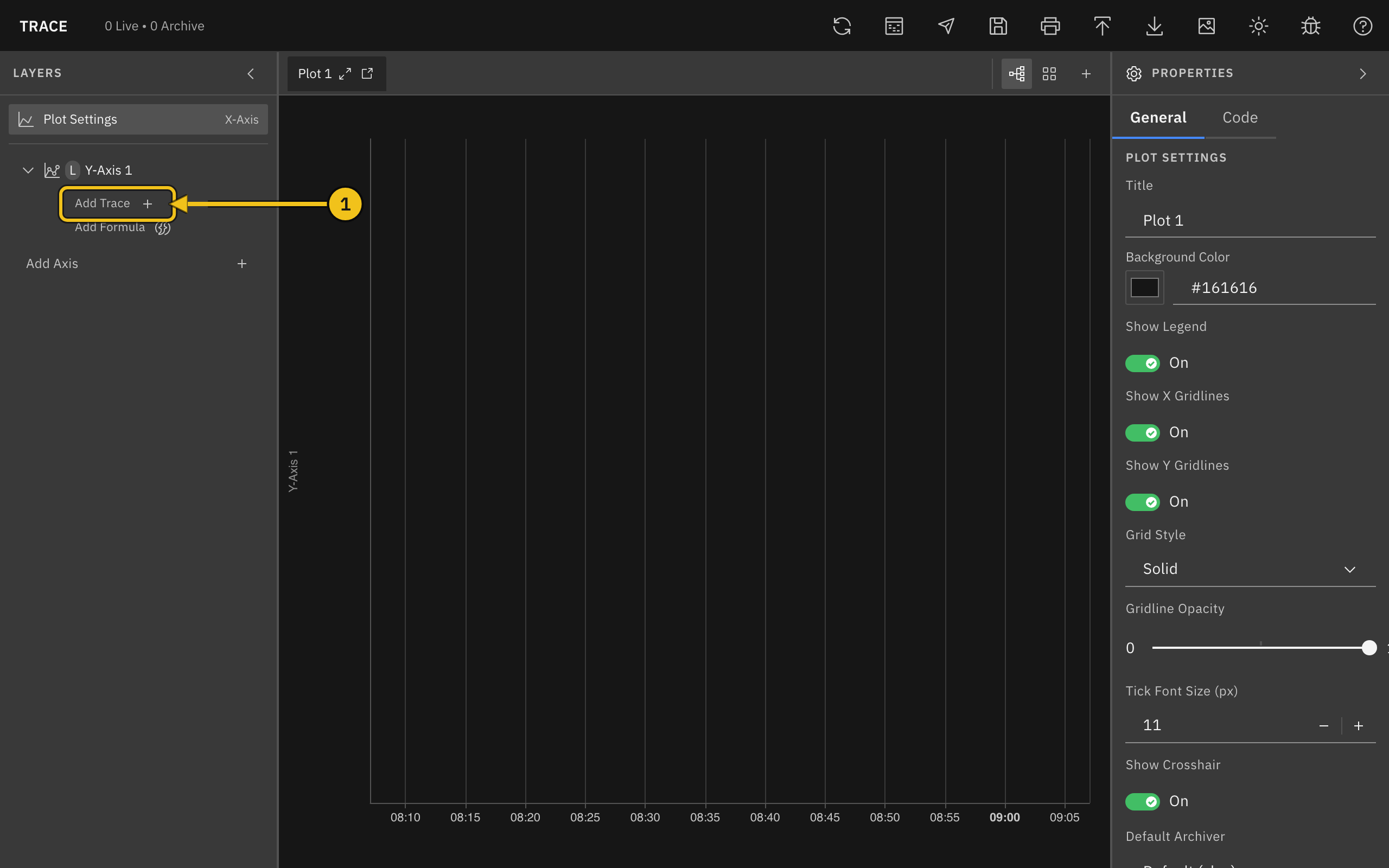
- In the Layers panel on the left, click Add Trace under the axis you want to use (①). The new trace is selected, and its settings open in the Properties panel on the right.
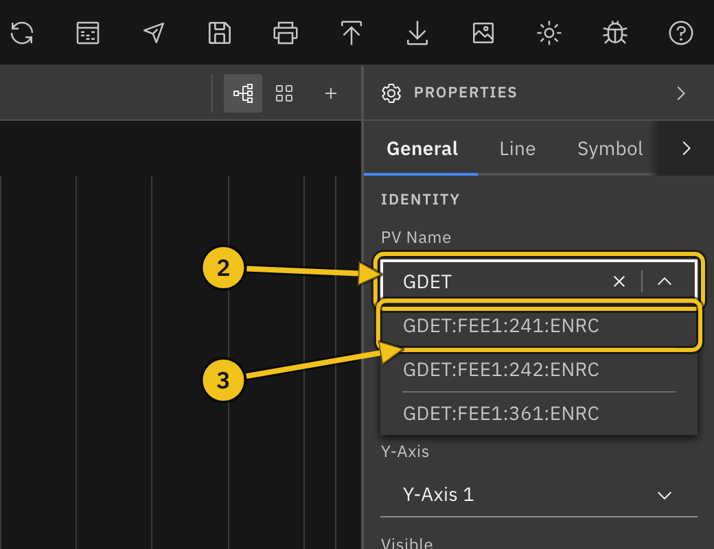
- Click the PV Name field and type part of the PV name (②). Matching PVs from the archiver appear in a list as you type.
- Click the PV you want (③), or press Enter to use exactly what you typed.
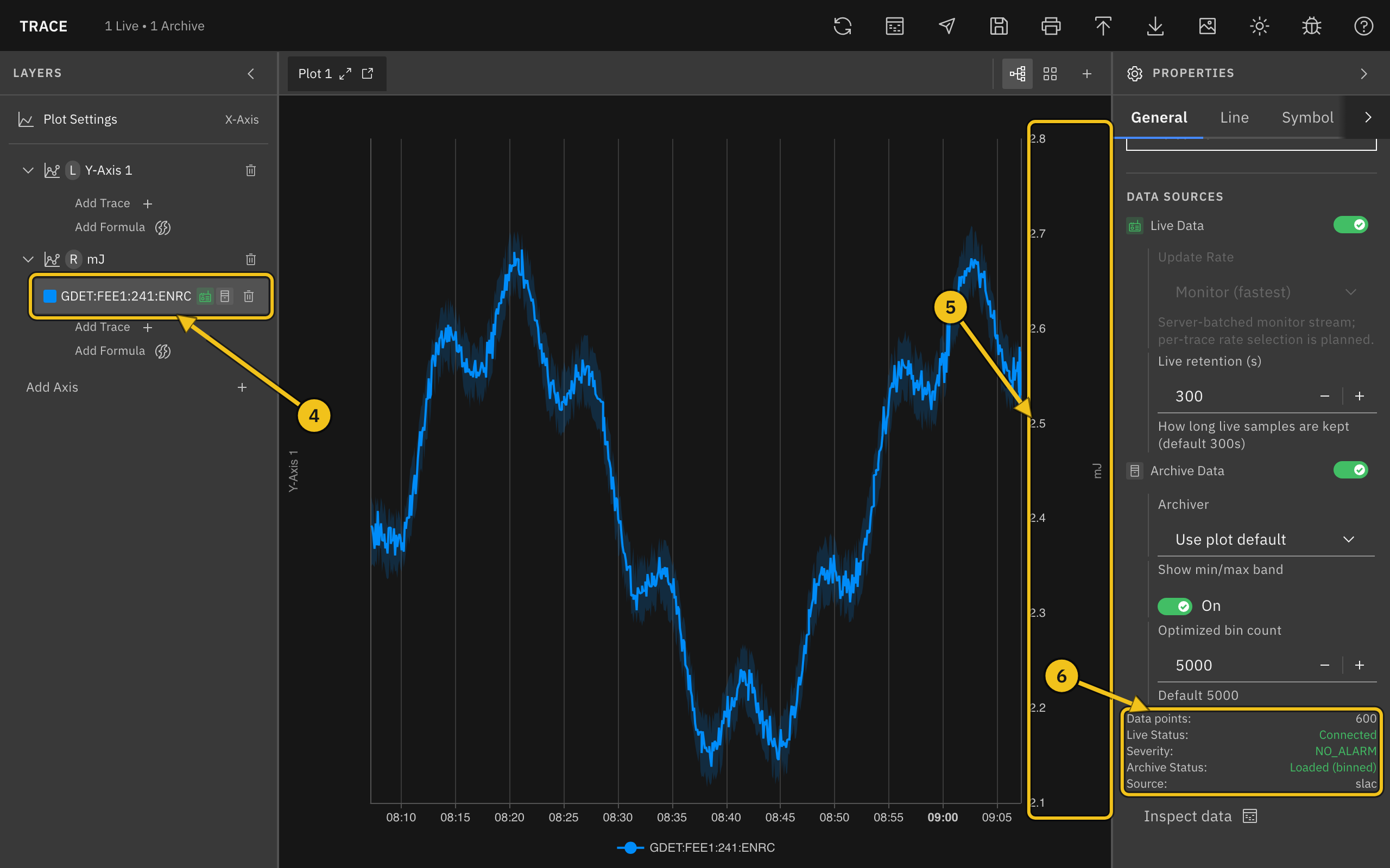
Once you choose a PV, the trace starts drawing:
- ④ Layers — the trace is listed under its axis, with icons showing that live and archive data are on. Click the row any time to edit the trace again.
- ⑤ Units axis — the trace moves to an axis named after the PV's units (here mJ). See Axes and Units.
- ⑥ Status — the bottom of the Data Sources section shows Live Status and Archive Status. Useful when a trace isn't drawing and you want to know why.
Add Several PVs at Once
To add many PVs in one go, click the Search PVs icon in the header, or the Search PVs button below a plot's axes in the Layers panel.
- Type part of a PV name in Pattern. Matches from the archiver appear as you type.
*matches any run of characters and?matches one, soKLYS:LI2*:PDESfinds every PV that starts withKLYS:LI2and ends with:PDES. - Tick the PVs you want, or use Select all at the top of the list. Matches are listed alphabetically. Ticks are kept when you change the pattern, so you can gather PVs from several searches; the Selected row shows them and lets you remove one or clear them all.
- Click Add N PVs. Double-clicking a match adds it straight away, together with anything already selected.
The new traces appear under the plot's first axis and move to their units axes as the lookups finish (see Axes and Units). PVs that are already on the plot are marked on plot; you can still add them again. The dialog lists at most 500 matches, so narrow the pattern if the PV you want isn't shown. With more than one plot open, the dialog starts on the current plot and Add to plot lets you pick another.
Axes and Units
When you choose a PV, Trace looks up its engineering units and moves the trace to the axis with the same units. If there isn't one, Trace creates a new axis named after the units, alternating between the left and right sides of the plot. Traces with the same units share an axis, so they are easy to compare.
You can always move a trace yourself: pick a different axis from the Y-Axis dropdown, or drag the trace onto another axis in the Layers panel. The original Y-Axis 1 stays even when it is empty; click its trash icon to remove it if you don't need it.
Note: A newly created axis currently starts collapsed in the Layers panel. Click the chevron next to the axis name to see its traces.
Live and Archive Data
Data sources:
- Live Data — streams new values as they arrive. Live retention (s) sets how much live history is kept (default 300 seconds).
- Archive Data — loads the plot's time range from the archiver. For ranges longer than 30 minutes, the archiver returns averaged bins, and Trace draws a shaded min/max band behind the line. Turn the band off with Show min/max band.
With both on, archive data covers the past and live data takes over from the last archived sample. Each trace uses the plot's Default Archiver unless you choose a different one under Archiver.
When a Trace Doesn't Draw
Check the status lines at the bottom of Data Sources, or the label next to the trace in the Layers panel. Hover over a label to see the full error.
- Disconnected (Live Status) — the live connection dropped. Trace reconnects on its own.
- Waiting for value (Live Status) — connected, but no value has arrived for this PV yet.
- Unknown PV — the archiver has no PV with that name. Check the spelling in PV Name.
- No archiver — no archiver is set for this plot. Choose one in the plot's Default Archiver setting or the trace's Archiver setting.
- Archiver down, Timeout, or Offline — the archiver or network isn't responding. Click the refresh icon in the header to try again.
Set the Time Range
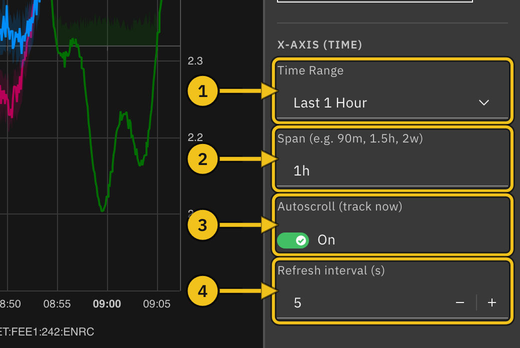
Each plot has its own time range. Select Plot Settings in the Layers panel, then scroll to X-Axis (Time) in the Properties panel.
Time settings:
- ① Time Range — choose a preset from Last 1 Hour to Last 1 Month, or Custom Range... for fixed start and end times.
- ② Span — type any length of time, such as
90m,1.5h, or2w, and press Enter. Units arem(minutes),h(hours),d(days),w(weeks), andM(months). - ③ Autoscroll (track now) — keeps the current time at the right edge of the plot.
- ④ Refresh interval (s) — how often, from 1 to 60 seconds, the plot moves forward while autoscroll is on.
Custom Range
Choose Custom Range..., then set From and To. Leave To blank to end the range at the current time. If the range isn't valid (for example, From is after To), an error appears below the fields and the plot shows the last hour instead.
Returning to the Full Range
Autoscroll turns off by itself when you zoom or pan the plot. To return to the full time range and follow the current time again, choose a different Time Range or enter a different Span. To keep the same range, choose another one and then switch back.
Note: Switching Autoscroll back on, or re-entering the same Span, does not undo a zoom or pan. Change the range as described above.
Zoom, Pan, and Read Values
Mouse controls:
- Scroll inside the plot — zoom the time axis in or out.
- Drag inside the plot — move along the time axis.
- Scroll over a Y-axis (②) — zoom only that axis, around the mouse pointer.
- Drag up or down on a Y-axis — move only that axis.
Zooming or panning time turns off autoscroll (see Returning to the Full Range). Zooming or panning a Y-axis switches it from Auto Scale to fixed limits; turn Auto Scale back on in the axis settings to undo it.
Move the mouse over the plot to see a tooltip (①) with each trace's value at that time. Each value is the sample nearest the pointer, and the time in parentheses shows how far that sample is from the pointer (for example +2s). Turn Show Crosshair off in Plot Settings to hide the dashed crosshair lines; the tooltip still appears.
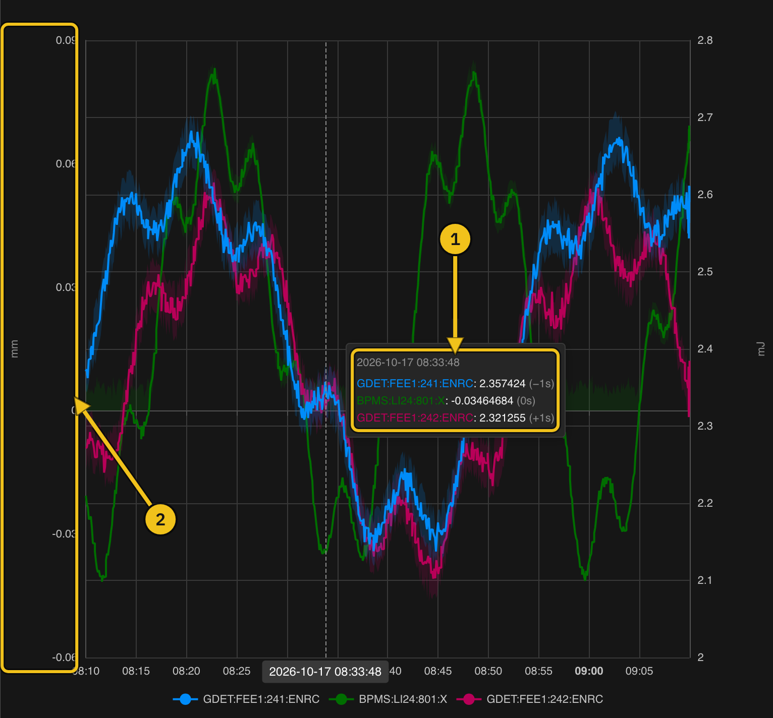
The legend below the plot lists the visible traces. Clicking it doesn't hide a trace; use the Visible switch in the trace's settings instead.
Work with Axes
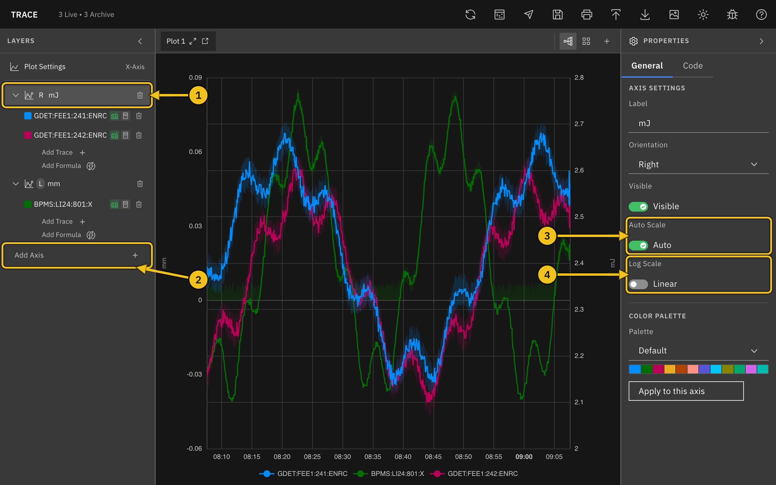
A plot can have several Y-axes, each with its own scale, on the left or right side. Traces with different units usually go on different axes.
Workflow:
- In the Layers panel, click Add Axis (②) below the plot's axes. New axes alternate between the left and right sides.
- Click the axis row (①) to open its settings in the Properties panel.
Axis settings:
- Label — the axis name shown in Layers and along the axis.
- Orientation — Left or Right.
- Visible — show or hide the axis. Hiding an axis also hides its traces.
- Auto Scale (③) — fit the axis to the data. Turn it off to set Min Value and Max Value yourself; they start from the range currently shown.
- Log Scale (④) — switch between a linear and a logarithmic scale.
Move Traces Between Axes
Drag a trace in Layers onto another axis, or pick an axis from Y-Axis in the trace's settings. In grid view, you can also drag a trace onto an axis in another plot.
Delete an Axis
Click the trash icon on the axis row. Its traces move to another axis on the same plot. A plot always keeps at least one axis.
Note: Deleting an axis, trace, or plot happens immediately, without asking for confirmation.
Style Traces
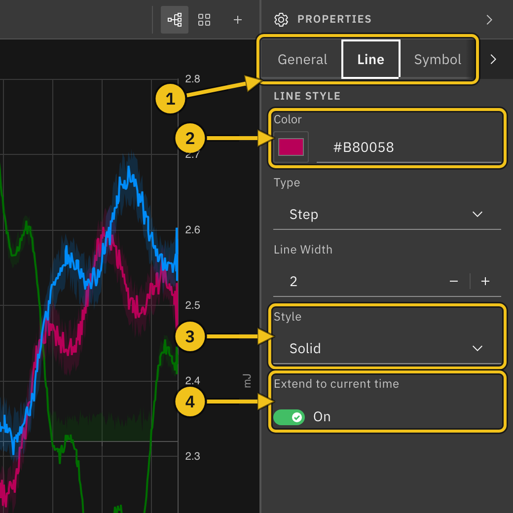
Select a trace in Layers to change how it looks. On the General tab, Display Name sets the name used in the legend, tooltip, and Layers (leave it blank to use the PV name), and Visible shows or hides the trace.
Line tab:
- ① Tabs — switch between General, Line, Symbol, and Code. If the panel is narrow, use the arrow at the end of the tab row to reach Code.
- ② Color — pick a color or type a hex value.
- Type — Step (holds each value until the next sample; the default) or Direct (straight lines between samples).
- Line Width — 1 to 5.
- ③ Style — solid, dashed, dotted, and mixed patterns, or NoLine to show only symbols.
- ④ Extend to current time — draw a dashed line from the last value to the end of the time range.
On the Symbol tab, turn on Show Symbols to mark each sample, then choose a Shape and Size.
Note: The Code tab is a preview of the chart settings behind the trace. Its Apply Changes and Format buttons don't do anything yet.
Color Palettes
New traces get their colors from a palette. Select Plot Settings and scroll to Color Palette:
- ① Palette — choose one of 13 palettes. New traces on every plot use it from then on, and Trace remembers your choice.
- ② Apply to all traces — recolor every trace on this plot from the palette.
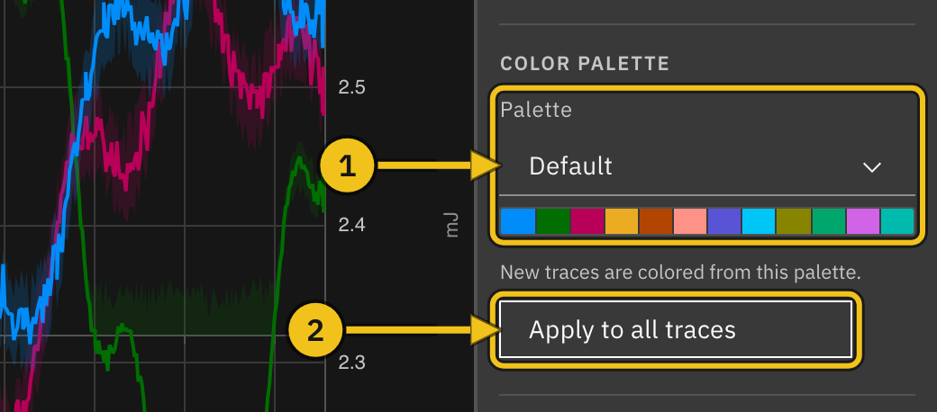
To recolor only one axis's traces, select the axis and use Apply to this axis in its Color Palette section. Choosing a palette there doesn't change the palette for new traces.
Formulas
A formula curve calculates new values from other traces, for example the ratio of two detectors or a scaled copy of a signal.
Workflow:
- Click Add Formula (①) under the axis where the result should appear. The new curve (④) is added to that axis and selected.
- Enter a Display Name.
- Type an expression in the Formula box (②). Refer to other traces with variables in braces, such as
{x1}and{x2}. Trace checks the expression as you type and shows Valid or an error. - Under Variables (③), choose the trace each variable stands for.
- The curve draws once every variable is bound.
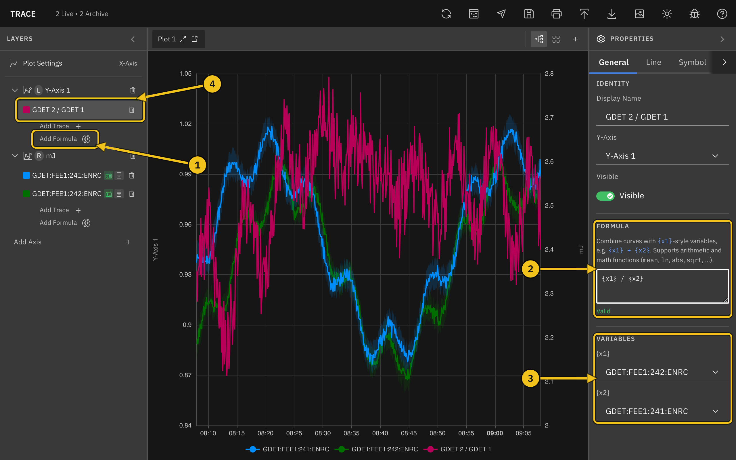
Expressions support arithmetic (+, -, *, /, and parentheses) and math functions such as mean, ln, abs, and sqrt. For example, {x1} * 1.5 + 10.
Formula curves are recalculated whenever the plot's time range moves, including with autoscroll.
Create a Formula from a Trace
Select a PV trace and click Create formula from this curve in the Derived section. Trace adds a formula curve with {x1} already bound to that trace; edit the expression from there. The original trace is unchanged.
Note: Variables can refer only to PV traces on the same plot, not to other formulas.
Multiple Plots
Add more plots to view different groups of PVs side by side. Each plot has its own axes, traces, time range, and settings.
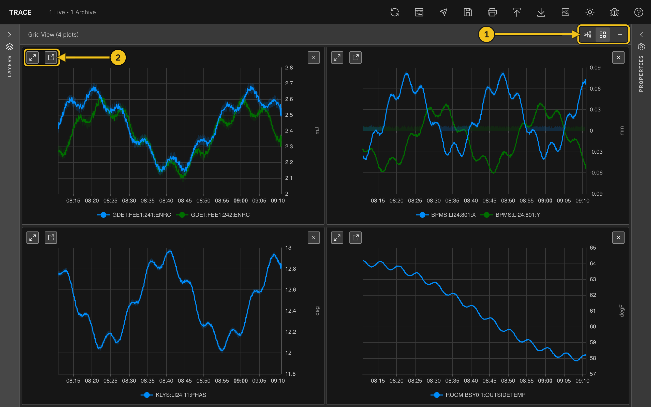
View controls (①, at the right end of the tab bar):
- Tab view — show one plot at a time, with a tab for each plot.
- Grid view — show all plots at once.
- Add plot (+) — add a new, empty plot and switch to it.
Managing plots:
- Rename a plot — select Plot Settings and edit Title.
- Close a plot — click × on its tab, or in the corner of its grid cell. This appears only when there is more than one plot.
In grid view, the Layers panel lists every plot, so you can edit any of them and drag traces between plots.
Fullscreen and Separate Windows
Each plot tab and grid cell (②) has two more buttons:
- Fullscreen — show the plot over the whole window. Click × in its title bar to return (Escape doesn't close it).
- Detach to window — move the plot into its own browser window. Useful with a second monitor. Click Reattach in that window, or close it, to bring the plot back.
Note: If your browser blocks pop-up windows, the plot stays in the main window. Allow pop-ups for Trace to detach plots.
Inspect Data
The Data Insight tool lists a PV's samples in a table. Useful when you need exact values and timestamps, or want to export one PV's data.
Open it by:
- Clicking the Data Insight icon in the header (Option+D on macOS, Alt+D elsewhere)
- Clicking Inspect data at the bottom of a trace's Data Sources settings
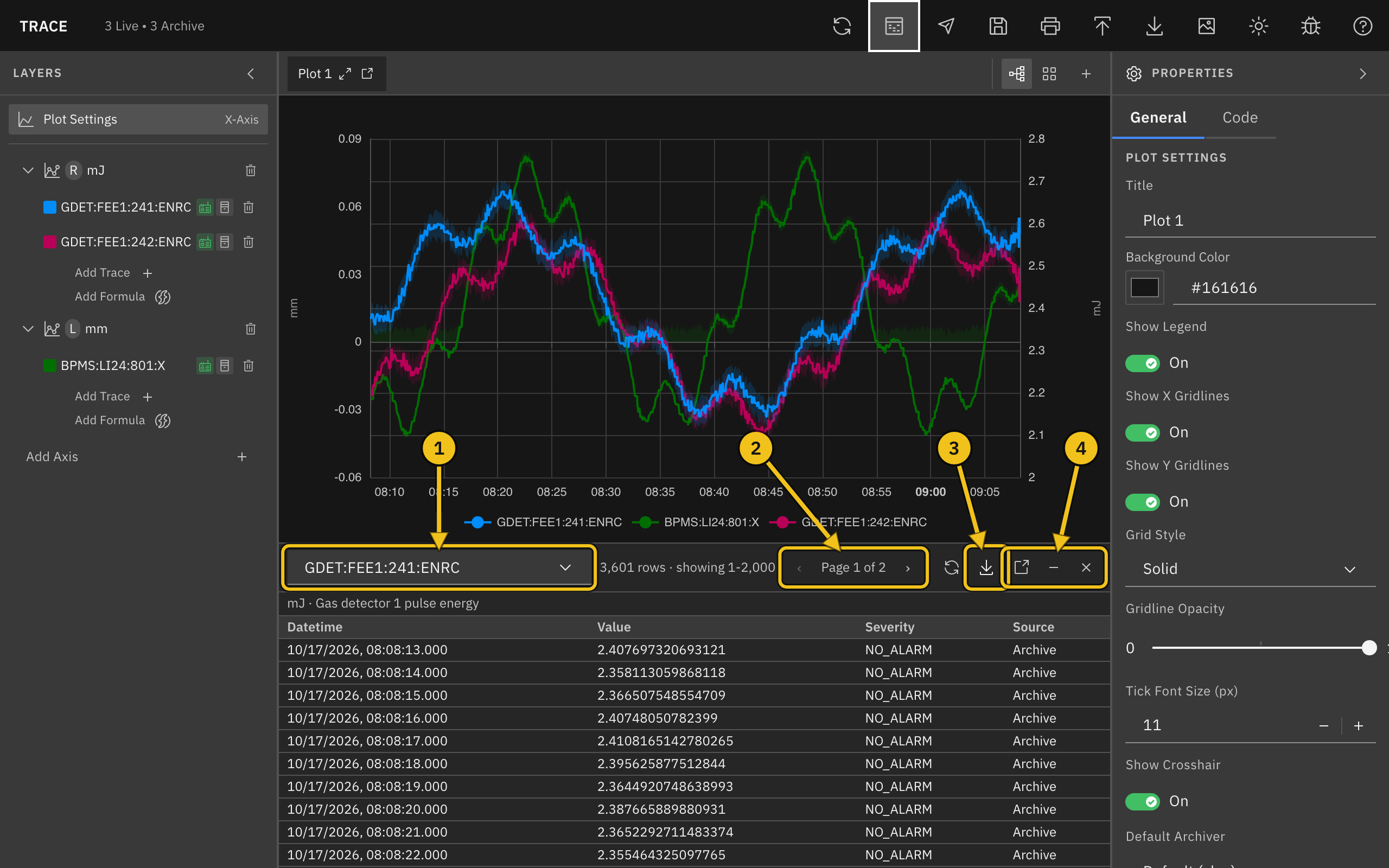
Controls:
- ① PV — choose which PV to inspect. In grid view, the list includes PVs from every plot.
- ② Pages — the table shows 2,000 rows per page; use the arrows to move between pages.
- ③ Export — download all rows as CSV, JSON, or MAT (MATLAB). Exports include the PV name, units, and description.
- ④ Pop out, Minimize, Close — move the tool into its own window, shrink it to a bar below the plot, or close it.
The refresh icon to the left of Export loads the data again.
The table covers the plot's current time range and shows each sample's Datetime (to the millisecond), Value, Severity, and Source (Archive or Live). The PV's units and description appear above the table. For very long ranges the archiver may thin out the samples; the row count then shows (decimated).
Save and Open Workspaces
A workspace stores your plots, axes, traces, styles, time ranges, and theme. It doesn't store data; Trace loads the data again when you open the workspace.
- Save (Cmd+S / Ctrl+S) — click the save icon in the header to download the workspace as a
.trc.jsonfile. - Import (Cmd+O / Ctrl+O) — click the import icon and choose a workspace file. It replaces whatever is open.
Trace can also open .trc files from the older PyDM-based Trace. Settings that have no equivalent are skipped, and Trace lists them in a message after importing.
Note: Importing replaces the current workspace without asking. Save first if you want to keep it.
Export and Print
- Export CSV — downloads one CSV file per plot, named after the plot title. Each row has the PV name, the time (in nanoseconds and as a date), and the value. Archive and formula data are included; traces with only live data are not. For ranges longer than 30 minutes, the archive values are the averaged bins shown on the plot.
- Export PNG (Cmd+I / Ctrl+I) — downloads an image of each plot on screen: the active plot in tab view, every plot in grid view, or the fullscreen plot.
- Print (Cmd+P / Ctrl+P) — prints the plots on screen, arranged in a grid on the page.
Plots detached into separate windows are left out of PNG exports and printouts.
Post to E-Log
Click the E-Log icon in the header (Cmd+E / Ctrl+E) to post the plots on screen to the E-Log. The icon appears only when Trace is connected to an E-Log.
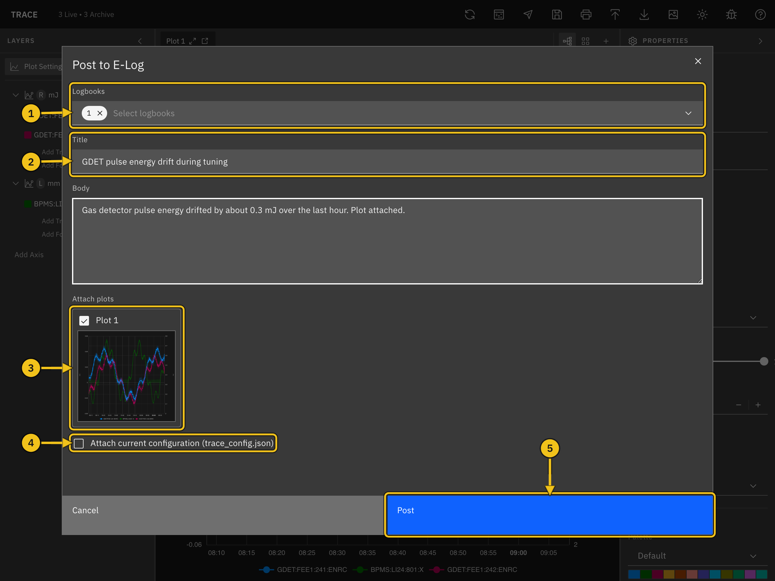
Workflow:
- Choose one or more Logbooks (①).
- Enter a Title (②) and, optionally, a Body.
- Under Attach plots (③), clear any plot you don't want to include. The images are taken when the dialog opens: the active plot in tab view, or every plot in grid view.
- Check Attach current configuration (④) to add the workspace as
trace_config.json, so others can open the same view in Trace. - Click Post (⑤). A message in the top-right corner confirms the new entry.
Keyboard Shortcuts
| Action | macOS | Windows / Linux |
|---|---|---|
| Save workspace | Cmd+S | Ctrl+S |
| Import workspace | Cmd+O | Ctrl+O |
| Cmd+P | Ctrl+P | |
| Export PNG | Cmd+I | Ctrl+I |
| Post to E-Log | Cmd+E | Ctrl+E |
| Data Insight | Option+D | Alt+D |
| Switch light/dark mode | Option+T | Alt+T |
Shortcuts don't run while you are typing in a text field.
Icons and Tooltips
Every icon in Trace has a tooltip that appears on hover. Here's a quick reference:
| Icon | Meaning |
|---|---|
 | Refresh archive data |
 | Open Data Insight |
 | Post to E-Log |
 | Save workspace |
 | |
 | Import workspace |
 | Export CSV |
 | Export PNG |
 | Switch between light and dark mode |
 | Report a bug |
 | Open the documentation |
 | Show the plot fullscreen |
 | Detach the plot to its own window |
 | Close the plot |
 | Tab view |
 | Grid view |
 | Add a plot |
 | Trace uses live data |
 | Trace uses archive data |
 | Delete the trace or axis |
Dark Mode
Click the sun/moon icon in the header (Option+T / Alt+T) to switch between dark and light mode. Your choice is saved in the browser and used on future visits. Plots with the default background follow the theme; a plot with a custom Background Color keeps it.
Getting Help
Click the bug icon in the header to report a problem or request a feature. See Support and Contact Information for what to include.